Probabilistic Reasoning Over Time¶

Up to now, agents we have worked with, used their current data provided by their sensors to choose their action. Yet, they have much more than that. They've seen the past. In this chapter we will talk about agents that can perceive the world their in, how it works, and can quantify the degree of belief they have in their perception.

Time and Uncertainty¶

Let's discuss the change we're making to the scope of problems we're solving. We have developed our techniques for probabilistic reasoning in the context of static worlds, in which each random variable has a single fixed value. For example, when repairing a car, we assume that whatever is broken remains broken during the process of diagnosis; our job is to infer the state of the car from observed evidence, which also remains fixed.

Now consider a slightly different problem: treating a diabetic patient. As in the case of car repair, we have evidence such as recent insulin doses, food intake, blood sugar measurements, and other physical signs. The task is to assess the current state of the patient, including the actual blood sugar level and insulin level. Given this information, we can make a decision about the patient’s food intake and insulin dose. Unlike the case of car repair, here the dynamic aspects of the problem are essential. Blood sugar levels and measurements thereof can change rapidly over time, depending on recent food intake and insulin doses, metabolic activity, the time of day, and so on. To assess the current state from the history of evidence and to predict the outcomes of treatment actions, we must model these changes.

The same considerations arise in many other contexts, such as speech recognition, robot localization, user attention, medical monitoring, etc.

States¶

We view the world as a series of snapshots, or time slices, each of which contains a set of random variables. (Uncertainty over continuous time can be modeled by stochastic differential equations, SDEs. The models studied in this chapter can be viewed as discrete-time approximations to SDEs.)

To model our problems, we first start with Markov chains, and will continue to adopt it to better meet our real world requirements.

Markov Chain¶

A Markov process is a stochastic process that satisfies the Markov property (sometimes characterized as memorylessness). In simpler terms, it is a process for which predictions can be made regarding future outcomes based solely on its present state and—most importantly—such predictions are just as good as the ones that could be made knowing the process's full history. In other words, conditional on the present state of the system, its future and past states are independent.

A Markov chain is a type of Markov process that has either a discrete state space or a discrete index set (often representing time), but the precise definition of a Markov chain varies. Here, we use Markov chains that have a time as their discrete index set.

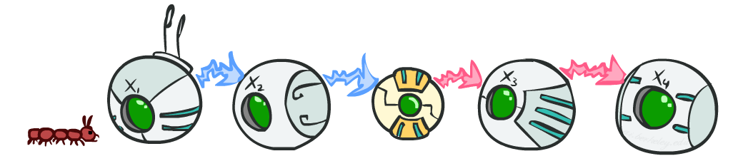
We define $X_t$ the state of the world in out problem at time $t$, i.e. $t$th snapshot we have.

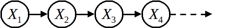
As we said before, $X_t$ relies only on $X_{t-1}$, so the bayes net for a Markov chain would be as the above figure.

We define transition probabilities or dynamics, the CPT of $X_i|X_{i-1}$. Doing this, we have made an assumption about how the states are evolving, transition probabilities are the same at all times. This is called stationary assumption.

We can define this Markov chain, using its initial state probabilities, i.e. the CPT of $X_1$, and transition probabilities.

Like we learned before, we can calculate the joint distribution as:

\begin{align*} P(X_1, X_2, ..., X_T) &= P(X_1)P(X_2|X_1)P(X_3|X_2)...P(X_T|X_{T-1}) \\ &= P(X_1) \prod_{i=2}^T{P(X_i|X_{i-1})} \end{align*}

This represents the probability of a sequence of events. We can use this measure to quantify how likely the world we perceived is.

Remember this model relies on the Markov property we mentioned earlier. Obviously, if this assumption is far-fetched, we have to make a more complex bayes net, and thus, the resulting joint distribution would have been different.

The most general formula we can write for a process, is when we take into account the effect of every previous state, i.e.

\begin{align*} P(X_1, X_2, ..., X_T) &= P(X_1)P(X_2|X_1)P(X_3|X_2, X_1)...P(X_T|X_{T-1},...,X_1) \\ &= P(X_1) \prod_{i=2}^T{P(X_i|X_{i-1},...,X_1)} \end{align*}

You can simply prove that the two statements are equal, when $X_i \perp X_{i-2},...,X_1 | X_{i-1}$.

Example¶

Let's have an example to clear the air. We assume that changes of the weather is a Markov process, i.e. its state relies solely on its last step. So we make our snapshots everyday. We also that weather is classified into two states, namely rain and sun. Moreover, the initial state probabilities are defined by:

state	probability
sun	1.0
rain	0.0

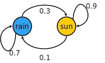
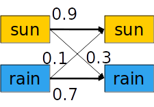
And we assume that the dynamics for this problem are:

X_{t-1}	X_t	P(X_t\	X_{t-1})
sun	sun	0.9
sun	rain	0.1
rain	sun	0.3
rain	rain	0.7

We can also, represent this CPT as depicted by figures below.

* What is probability distribution after one step? (Click for solution!)

\begin{align*} P(X_2=sun) &= P(X_2=sun|X_1=sun)P(X_1=sun) + P(X_2=sun|X_1=rain)P(X_1=rain) \\ &= 0.9 \times 1.0 + 0.1 \times 0.0 = 0.9 \end{align*}

* What's $P(X)$ on some day $t$? (Click for solution!)

To answer this question, we use mini-forward algorithm, introduced below.

Mini-Forward Algorithm¶

The problem we're trying to find solution for in this algorithm is the value of $P(X)$ on some day $t$. Mini-Forward Algorithm uses dynamic programming to find answer for this question.

$P(X_1)$ is known to us. We successively calculate probability of $P(X_t)$.

\begin{align*} P(X_t) &= \sum_{x_{t-1}} P(x_{t-1}, x_t) \\ &= \sum_{x_{t-1}} P(x_t|x_{t-1})P(x_{t-1}) \end{align*}

This is like we are simulating the transition for every day.

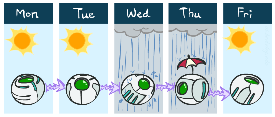
An execution of this algorithm up to $t=4$ has been done below.

Let's put it into code.

Next, we want to calculate the state's probabilities for $t=10000$ with several initial states.

It seems like no matter what initial value we choose, we end up with days that are 75% sunny. (Go ahead and test some initial values of your own.

Stationary Distributions¶

A stationary distribution is a specific entity which is unchanged by the effect of some matrix or operator.

Regarding our topic, it's a special distribution for a Markov chain, such that if the chain starts with its stationary distribution, the marginal distribution of all states at any time will always be the same stationary distribution. Assuming irreducibility, the stationary distribution is always unique if it exists.

For most chains, influence of the initial distribution gets less and less over time and the distribution we end up in is independent of the initial distribution. This is the so-called stationary distribution. Note that regarding its definition, it satisfies:

$$P(X_\infty) = P(X_{\infty +1}) = \sum_x P(X|x)P(X_\infty)$$

Example¶

Let's prove that for the previous example, the stationary distribution is really what we guessed.

\begin{cases} P_\infty(sun) = P(sun|sun)P_\infty(sun) + P(sun|rain)P_\infty(rain) \\ P_\infty(rain) = P(rain|sun)P_\infty(sun) + P(rain|rain)P_\infty(rain) \end{cases}

\begin{cases} P_\infty(sun) = 0.9P_\infty(sun) + 0.3P_\infty(rain) \\ P_\infty(rain) = 0.1P_\infty(sun) + 0.7P_\infty(rain) \end{cases} \begin{cases} P_\infty(sun) = 3P_\infty(rain) \\ P_\infty(rain) = \frac{1}{3}P_\infty(sun) \end{cases}

Note that $P_\infty(sun) + P_\infty(rain) = 1$, thus

\begin{align*} \begin{cases} P_\infty(sun) = 0.75 \\ P_\infty(rain) = 0.25 \end{cases} Q.E.D \end{align*}

Applications¶

Web Link Analysis¶

Assume we use web pages as our state. We start from a uniformly random web page, and in each step change the state to some other uniformly random web page with probability $c$, and follow a random outlink in the web page with probability $1-c$.

It can be seen that we'll spend more time on web pages that are highly reachable. e.g. since many sites use Flash, you can probably find a path from any site to Acrobat Flash download page.

In fact, since this transitions are random, leading it to a certain site, requires making path from many sites to it, which is practically impossible, so it's somewhat robust to link spam.

Google 1.0 returned the set of pages containing all your keywords in decreasing rank (the time spent on that web page). Nowadays, all search engines use link analysis along with many other factors. (rank is actually getting less important over time)

Gibs Sampling¶

We define:

• Each state as a set of all random and query variables, i.e. $\{X_1,...,X_n\} = H \cup Q$
• Transitions as resampling one of the variables regarding all its parents, i.e we resample $x$ according to: $$P(X_i|X_1,X_2,...X_n, E_1, ..., E_m)$$ Where $E_i$ is an evidence.

As the time passes by our state will converge to a valid state regarding the problem's Bayes net.

Hidden Markov Model¶

Usually if we look at the problem's input, it doesn't yield a Markov chain. But still, there is hope.

If the problem has a superior state that is a Markov process, we can make an assumption about this superior state, our belief, and update it as we observe problem's inputs.

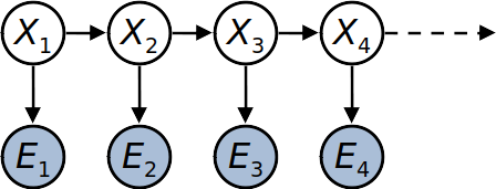
To model this system, we start with a simple Markov chain, and at each state, add a new node for the inputs of the problem such as agent's sensors, etc. which is solely relied on its state (i.e. $P(E_t|X_{0:t},E_{0:t-1}) = P(E_t|X_t)$. This property is called sensor Markov assumption).

You can see a sample Hidden Markov Model (HMM) above.

Example¶

Let's use the weather problem to clear the air again. Imagine that you are the security guard stationed at a secret underground installation. You want to know whether it’s raining today, but your only access to the outside world occurs each morning when you see the director coming in with, or without, an umbrella. For each day $t$, the set $E_t$ thus contains a single evidence variable $Umbrella_t$ or $U_t$ for short (whether the umbrella appears), and the set $X_t$ contains a single state variable $Rain_t$ or $R_t$ for short (whether it is raining).

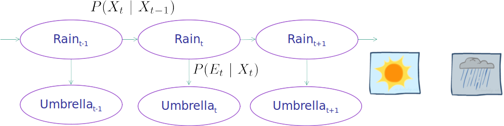
This Bayes net can help us to find whatever query we have.

Joint Distribution of an HMM¶

Like Markov chain, we write the joint distributions of all variables: \begin{align*} P(X_1, E_1, ... ,X_T, E_T) &= P(X_1)P(E_1|X_1) \prod_{t=2}^T P(X_t|X_{t-1:0})P(E_t|X_{t:0}) \\ &= P(X_1)P(E_1|X_1) \prod_{t=2}^T P(X_t|X_{t-1})P(E_t|X_t) \end{align*}

Note how we used the sensor Markov assumption along with Markov property to simplify the result.

You remember from before that the sensor Markov assumption is $E_i \perp X_{i-1},...,X_1, E_{i-1},...,E_1 | X_{i}$.

Applications¶

Speech Recognition HMMs¶

Hidden Markov Models (HMMs) provide a simple and effective framework for modelling time-varying spectral vector sequences. As a consequence, almost all present day large vocabulary continuous speech recognition (LVCSR) systems are based on HMMs.

We use acoustic signals as our observation, and specific positions in words as our states (so we have tens of thousands of states).

Machine Translation HMMs¶

On a basic level, machine translation performs mechanical substitution of words in one language for words in another, but that alone rarely produces a good translation because recognition of whole phrases and their closest counterparts in the target language is needed. Not all words in one language have equivalent words in another language, and many words have more than one meaning.

Here, we observe words, and our states are translation options.

Robot Tracking¶

In this application, we want to localize a robot using the range readings its sensors provide. (sesors provide our observation)

Here, states are possible possitions of the robot on the map.