Temporal Probability Models (Markov Models and Particle Filtering)

Robot Localization¶

In robot localization, we know the map, but not the robot’s position. An example of observations would be vectors of range finder readings, this means our agent has a couple of sensors, each reporting the distance in a specific direction with an obstacle. State space and readings are typically continuous (works basically like a very fine grid) and so we cannot store $B(X)$. Due to this property of problem, particle filtering is a main technique.

So, we use many particles, uniformly distributed in the map. Then, after each iteration, we become reluctant to those of them that do not have probable readings. As a result, trusting that map would have been different to the eyes of our particles, we would end up with our particles centered at the real position.

The below depiction shows this perfectly. The red dots represent particles. Notice how the algorithm can't decide between two positions until entering a room.

What algorithm do you think would be better to drive the agent with, so that we can find and benefit from asymmetries in the map? (Think about random walks)

We can even even go a step further, and forget about the map. This problem is called Simultaneous Localization And Mapping or SLAM for short. In this version of problem, we neither do know where the agent is, nor know what the map is. We have to find them both.

To solve this problem, we extend our states to also cover the map. For example, we can show our map with a matrix of 1s and 0s where every element is 1 if the map is blocked in the corresponding region on the map.

To solve this problem we use Kalman filtering and particle methods.

Notice how the robot starts with complete certainty about its position, and as the time goes on, it doubts if the position indeed is probable if it was a little bit away from its current position (like the readings would have been close to what they are now) and this leads to uncertainty even about the position. When the agent reachs a full cycle, it understands that it should be at the same position now, so its certainty about its position rises once again.

Dynamic Bayes Net¶

Dynamic Bayesian Networks (DBN) extend standard Bayesian networks with the concept of time. This allows us to model time series or sequences. In fact they can model complex multivariate time series, which means we can model the relationships between multiple time series in the same model, and also different regimes of behavior, since time series often behave differently in different contexts.

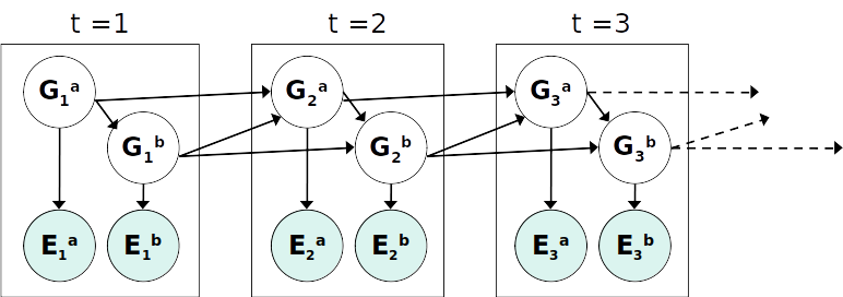
DBN Particle Filters¶

A particle is a complete sample for a time step. This is similar to reqgular filtering where we have to use sampling methods introduced earlier in the course instead of just a distribution.

Below are the steps we have to follow:

• Initialize

Generate prior samples for the $t=1$ Bayes net. e.g. particle $G_1^a = (3,3) G_1^b = (5,3)$ for above image.

• Elapse time

Sample a successor for each particle. e.g. successor $G_2^a = (2,3) G_2^b = (6,3)$

• Observe

Weight each entire sample by the likelihood of the evidence conditioned on the sample. Likelihood $p(E_1^a |G_1^a) \times p(E_1^b |G_1^b)$

• Resample

Select prior samples (tuples of values) in proportion to their likelihood.

Most Likely Explanation¶

We are introducing a new query, we can ask our temporal model. The query statement is as follows:

What is the most likely path of states that would have produced the current result.

Or more formally if our states are $X_i$ our observations are $E_i$, we want to find

$$argmax_{x_{1:t}} P(x_{1:t}|e_{1:t})$$

But how can we answer this query?

First, let's define the state trellis.

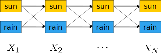
State trellis is a directed weighted graph $G$ that its nodes are the states, and an arc between two states $u$, and $v$ represents a transition between these two states. The weight of this arc is defined by the probablity of this arc happening. More formally, assume we have a transition between $x_{t-1}$ and $x_t$. Then the weight of the arc between these two will be $P(x_{t}|x_{t-1}) \times P(e_t|x_t)$

Note that with this definition, each path is a sequence of states, and the product of weights in this path is the probability of this path, provided the evidence.

Viterbi's Algorithm¶

Viterbi, uses dynamic programming model, to find the best path along the states. It first finds how probable a state at time $t-1$ is, and then reasons that the state at time $t$ relies solely on last state, and so having those probablities is enough to find the probability of new steps. Finally, the state that helps us find the most likely last state is it's parent.

\begin{align*} m_t[x_t] &= max_{x_{1:t-1}} P(x_{1:t-1}, x_t, e_{1:t}) \\ &= P(e_t|x_t)max_{x_{t-1}} P(x_t|x_{t-1})m_{t-1}[x_{t-1}] \end{align*}$$p_t[x_t] = argmax_{x_{t-1}} P(x_t|x_{t-1})m_{t-1}[x_{t-1}]$$

Example¶

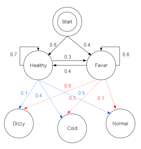
Consider a village where all villagers are either healthy or have a fever and only the village doctor can determine whether each has a fever. The doctor diagnoses fever by asking patients how they feel. The villagers may only answer that they feel normal, dizzy, or cold.

The doctor believes that the health condition of his patients operates as a discrete Markov chain. There are two states, "Healthy" and "Fever", but the doctor cannot observe them directly; they are hidden from him. On each day, there is a certain chance that the patient will tell the doctor he is "normal", "cold", or "dizzy", depending on his health condition.

The observations (normal, cold, dizzy) along with a hidden state (healthy, fever) form a hidden Markov model (HMM).

In this piece of code, start_p represents the doctor's belief about which state the HMM is in when the patient first visits (all he knows is that the patient tends to be healthy). The particular probability distribution used here is not the equilibrium one, which is (given the transition probabilities) approximately {'Healthy': 0.57, 'Fever': 0.43}. The transition_p represents the change of the health condition in the underlying Markov chain. In this example, there is only a 30% chance that tomorrow the patient will have a fever if he is healthy today. The emit_p represents how likely each possible observation, normal, cold, or dizzy is given their underlying condition, healthy or fever. If the patient is healthy, there is a 50% chance that he feels normal; if he has a fever, there is a 60% chance that he feels dizzy.

The patient visits three days in a row and the doctor discovers that on the first day he feels normal, on the second day he feels cold, on the third day he feels dizzy. The doctor has a question: what is the most likely sequence of health conditions of the patient that would explain these observations?