Uninformed Search
AI - Uninformed Search
Sharif University of Technology - Computer Engineering Department
Fateme Khashei, Hossein Sobhi, Ali asghar Ghanati
Probelm solving agents
Consider that we are currently in the city Arad, and have a flight leaving tomorrow from Bucharest. We need to find the shortest path from Arad to Bucharest so that we get there in time (a path is a sequence of cities, like: Arad, Sibiu, Fagaras, bucharest). An AI agent can help us achieve this goal (finding the best path) by using search algorithms.

Search strategies
A search strategy is defined by picking the order of node expansion, (expansion means visiting a node in a graph and generating its successors) strategies are evaluated by the following means:
- completeness: does it always find a solution if one exists?
- time complexity: number of nodes generated or expanded
- space complexity: maximum number of nodes held in memory
- optimality: does it find the best solution among all solutions?
- b: maximum branching factor of the search tree
- d: depth of the best solution
- m: maximum depth of the state space (may be infinity)
Uninformed Search
Uninformed search is a class of general-purpose search algorithms, used in different data structures, algorithms, and AIs.
Uninformed search algorithms do not have additional information about domain in which they are searching for a solution (mostly how far from the goal they are) other than how to traverse the tree, thats why they are called "uninformed".
Uninformed search algorithms are also called blind search algorithms. The search algorithm produces the search tree without using any domain knowledge, which is a brute force in nature. They don’t have any background information on how to approach the goal or whatsoever. But these are the basics of search algorithms in AI.
The diffrent type of search algorithms are as follows:

Breadth-First Search
Breadth-first search is the most common search strategy for traversing a tree or graph. This algorithm searches breadthwise in a tree or graph, so it is called breadth-first search.
BFS algorithm starts searching from the root node of the tree and expands all successor node at the current level before moving to nodes of next level.
In the below tree structure, you can see the traversing of the tree using BFS algorithm.

It starts from the root node of the tree which is 1, then goes to the next level and expands 2, we still have two nodes at this level so it expandss those two nodes which are 3 and 4, then there would be no successor left in this level so we can expand the next level and the proccess will be the same which gives us 5, 6, 7, 8 and for the last level we have 9, 10.
Completeness:
BFS is complete, which means if the shallowest goal node is at some finite depth, then BFS will find a solution.
Time complexity:
Time Complexity of BFS algorithm can be obtained by the number of nodes traversed in BFS until the shallowest Node.
Where the d = depth of shallowest solution and b is a node at every state.
T( b ) = b + b1 + b2 + ... + bd + b( bd - 1 ) = O( bd+1 )
Space complexity:
BFS algorithm requires a lot of memory space, because it keeps every node in memory.
Space complexity of BFS is O( bd+1 ).
Optimality:
In general, BFS is not optimal.
But BFS is optimal if path cost is a non-decreasing function of the depth of the node e.g. cost per step = 1.
Pseudocode:
function BFS (problem ,graph, source)returns soln/fail
    let Q be queue.
    Q.enqueue( source )
    mark source as visited
    while ( Q is not empty)
        node  =  Q.dequeue( )
        if Goal-Test(problem, State[node]) then return node
        for all successor in Expand(node, problem) do
            if successor is not visited
                Q.enqueue( successor )
                mark successor as visited.
    return failure
As you can see space is a big problem in this algorithm, it can easily generate nodes at 100MB/sec which means in 24 hours, 8640GB of data will be generated.
BFS will return shortest path in terms of number of transitions, It doesn’t find the least cost path.
This problem leads us to another search algorithm called Uniform Cost Search which is a generalization of BFS algorithm.
Uniform Cost Search
Uniform cost search, also called dijkstra, is a searching algorithm used for traversing a weighted tree or graph. This algorithm comes into play when a different cost is available for each edge.
The primary goal of the uniform cost search is to find a path to the goal node which has the lowest cumulative cost.
Uniformcost search expands nodes according to their path costs form the root node. It can be used to solve any graph or tree where the optimal cost is in demand. It gives maximum priority to the lowest cumulative cost.
Uniform cost search is equivalent to BFS algorithm if the path cost of all edges is the same.
It should be noted that UCS does not care about the number of steps involved in searching and only concerned about path cost. Due to which this algorithm may be stuck in an infinite loop.
In the below tree structure, you can see the traversing of the tree using UCS algorithm.
 The proccess of visiting the tree is similar to BFS except the fact that in BFS we use depth of the node to decide if we want to expand the node or not but in UFC we make the decision based on distance from root node.
In this example we have the root node and then the next level in the tree is consisted of yellow nodes, next green nodes and then purple ones and it goes like that till the end.
Completeness:
Uniform-cost search is complete, if a goal state exists, UCS will find it because it must have some finite length shortest path.
In other words, UCS is complete if the cost of each step exceeds some small positive integer, this to prevent infinite loops.
Time complexity:
Let C be cost of the optimal solution, and ε be each step to get closer to the goal node. Then the number of steps is C\/ε .
Hence, the worst-case time complexity of Uniform-cost search is O( bC\*/ε ).
Space complexity:
The same logic is for space complexity so, the worst-case space complexity of Uniform-cost search is O( bC\*/ε ).
Optimality:
Uniform cost search is optimal because at every state the path with the least cost is chosen.
Pseudocode:
function UCS (problem, graph, source)returns soln/fail
    for each successor in graph do
        Set-Infinity-Dist(successor)
    let Q be queue.
    Q.enqueue(graph)
    Dist[source] <- 0
    while ( Q is not empty)
        node = Get-Min-Dist(Q)
        Q.remove(node)
        if Goal-Test(problem, State[node]) then return node
        for all successor in Expand(node, problem) do
            Set-Dist(successor, node)
    return failure
This algorithm explores options in every direction because it doesn't have any information about goal location, this problem will be discussed in informed search chapter.
As we mentioned before space is a big problem in BFS and the problem still remains in UCS, to solve it we are going to talk about another search algorithm called Depth-First search.
Depth-First Search
Depth first search is a recursive algorithm for traversing a tree or graph that expands nodes in one branch as deep as the branch goes before expanding nodes in other branches.
It is called the depth-first search because it starts from the root node and follows each path to its greatest depth node before moving to the next path.
In the below tree structure, you can see the traversing of the tree using DFS algorithm.
 It starts from the root node which is 1 then expands a child and goes as deep as it can in the tree, so we get 2, 3 and 4 then it can't go any deeper so it expands another child which is 5 and perform DFS on this node which gives us 6, 7 and 8.
Proccess goes on until there is no node left.
Completeness:
DFS search algorithm is complete for graphs and trees in finite spaces (depths) as it will expand every node within a limited search tree.
DFS for graphs with cycles needs to be modified e.g. keeping the record of visited nodes to avoid processing a node more than once and getting caught in an infinite loop.
Time complexity:
Time complexity of DFS will be equivalent to the node traversed by the algorithm.
Let m = maximum depth of any node and this can be much larger than d (Shallowest solution depth).
Time complexity of DFS is O( bm ) time which is terrible if m is much larger than d.
Space complexity:
DFS algorithm needs to store only single path from the root node, hence space complexity of DFS is equivalent to the size of the fringe set, which is O(bm). ( linear space! )
Optimality:
DFS search algorithm is not optimal, as it may generate a large number of steps to reach to the solution.
Pseudocode:
function DFS (problem ,graph, source)returns soln/fail
    let S be stack.
    S.push( source )
    mark source as visited
    while ( S is not empty)
        node  =  S.pop( )
        if Goal-Test(problem, State[node]) then return node
        for all successor in Expand(node, problem) do
            if successor is not visited
                S.push( successor )
                mark successor as visited.
    return failure
So far we have introduced two algorithms:
- BFS which is better in time complexity
- DFS which is better in space complexity
we are looking for a way to combine strength of both in a method.
Depth Limited Search
A depth-limited search algorithm is similar to depth-first search with a with a depth limit.
Depth limited search is limited to depth l, which means that nodes at depth l will treat as it has no successor nodes further.
Depth-limited search can solve the drawback of the infinite path in the Depth-first search.
Completeness:
Depth-limited search algorithm is not complete, because it will not process nodes at depth deeper than l (depth limit).
Time complexity:
Time complexity of DLS algorithm is O( bl ).
Space complexity:
Space complexity of DLS algorithm is O( bl ).
Optimality:
Depth-limited search can be viewed as a special case of DFS, and it is also not optimal even if l > d. ( not complete means not optimal! )
Pseudocode:
function Depth-Limit-Search(problem, limit) returns soln/fail/cutoff
    Recursive-DLS(Make-Node(Initial-State[problem]), problem, limit)

function Recursive-DLS(node, problem, limit) returns soln/fail/cutoff
    cutoff-occured? <- false
    if Goal-Test(problem, State[node]) then return node
    else if Depth[node] = limit then return cutoff
    else for each successor in Expand(node, problem) do
        result <- Recursive-DLS(successor, problem, limit)
        if( ressult = cutoff ) then cutoff-occured? <- true
        else if( result != failure ) then return result
    if cutoff-occured? then return
Iterative Deepening Search
The iterative deepening algorithm is a combination of DFS and BFS algorithms. This search algorithm finds out the best depth limit and does it by gradually increasing the limit until a goal is found.
This algorithm performs depth-first search up to a certain "depth limit", and it keeps increasing the depth limit after each iteration until the goal node is found.
This Search algorithm combines the benefits of DFS's space-efficiency and BFS's completenessy.
The iterative search algorithm is useful uninformed search when search space is large, and depth of goal node is unknown.
In the below picture, you can see the traversing of a tree using iterative deepening algorithm.
 At first Limit is set to 0, it visits root node then limit is increased by 1 and we perform DFS for root and nodes with depth of 1.
for limit l, we perform DFS on nodes with maximum depth l and this goes on until we reach the goal.
Completeness:
Iterative deepening search is complete, which means if branching factor is finite, then it will find a solution.
Time complexity:
Let's suppose b is the branching factor and depth is d then the worst-case time complexity is:
T( b ) = (d+1)b0 + db1 + (d−1)b2 + ... + bd = O( bd )
or more percisely:
T( b ) = O( bd(1 – 1/b)-2 )
In this algorithm because of the fact that we want to avoid space problems, we wont store any data therefor we may have to repeat some actions but it won't trouble us because time complexity still remains O( bd ), similar to BFS.
Space complexity:
The space complexity of IDDFS will be O( bd )
Optimality:
IDDFS algorithm is optimal if path cost is a non-decreasing function of the depth of the node e.g. cost per step = 1.
Pseudocode:
function Iterative-Deepening-Search(problem) returns a solution
    inputs: problem, a problem
    for depth <- 0 to ∞ do
        result <- Depth-Limited-Search(problem, depth)
        if result ≠ cutoff then return result
    end
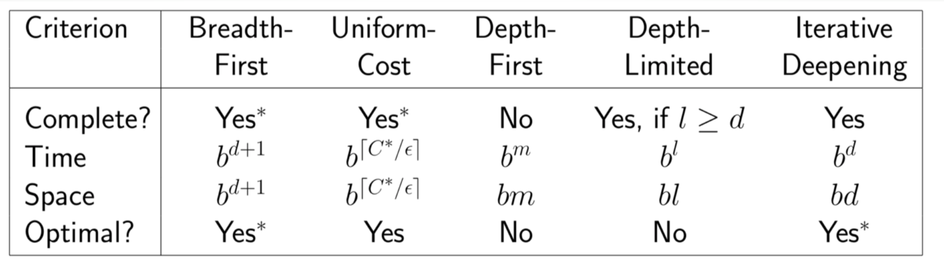
Summary of Algorithms
Refrences:
- AI course teached by Dr. Rohban at Sharif University of Technology, Spring 2021
- https://www.javatpoint.com
- https://www.analyticsvidhya.com
- https://www.geeksforgeeks.org
- https://www.wikipedia.org

Fatemeh Khashei
Hossein Sobhi
Ali Asghar Ghanati
