Courtesy: Most content are adopted from 15-780 course at CMU.

Continuous Optimization¶

In real life, we face a lot of problems with continues variables. Actually, the state of the environment, the way time is handled and the percepts and actions of agents might be continuous in our problems, in this section we provide an introduction to some local search techniques for finding optimal solutions in continuous spaces.

Examples¶

Weber Point¶

Given a collection of cities (assume on 2D plane) how can we find the location that minimizes the sum of distances to all cities? 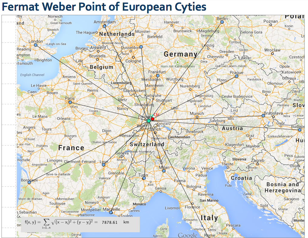Let's denote the location of cities as $y_1, y_2, ..., y_n$. Then we can find answer to our question by solving the optimization problem below: $$\min_{x} \sum^{n}_{i=1}||x-y_i||_2$$

Image deblurring and denoising¶

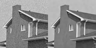Image Deblurring (Noise reduction) is the processes of removing blurring artifacts (noise) from images [input image say $Y$ which is blurred image which generally happens due to camera shake or some other phenomenon]. Given corrupted image $Y \in \mathbb R^{m\times n}$, we reconstruct the image by solving the optimization problem below: $$\min_X \sum_{i, j}|Y_{ij}-(K*X)_{ij}| + \lambda \sum_{i, j}\sqrt{(X_{ij}-X_{i, j+1})^2+(X_{i+1, j}-X_{ij})^2}$$ where $K*$ denotes convolution with a blurring filter.

Machine Learning¶

Virtually all (supervised) machine learning algorithms boil down to solving the optimization problem: $$\min_\theta \sum_{i=1}^m \ell(h_\theta(x_i), y_i)$$ where

• $x_i \in X$ are inputs
• $y_i \in Y$ are outputs
• $\ell$ is loss function
• $h_\theta$ is a hypothesis function parameterized by $\theta$

Optimization benefits¶

One of the key benefits of looking at problems in AI as optimization problems is that by doing so, we can separate out the definition of the problem and the method for solving it, and that way we can use general methods to solve different problems. There are off-the-shelf solvers for many classes of optimization problems that will let us solve even large, complex problems. We only need to put our problems in the right form.

Classes of optimization problems¶

There are many different types of optimization problems (linear programming, quadratic programming, nonlinear programming, semidefinite programming, integer programming, geometric programming, mixed linear binary integer programming, etc.). As these names could all get confusing, we instead classify problems by focusing on two dimensions:

• constrained vs. unconstrained
• convex vs. nonconvex

Constrained vs. Unconstrained¶

In an unconstrained optimization problem, every point $x \in \mathbb{R}^n$ is feasible, so we only focus on minimizing $f(x)$. In contrast, for constrained optimization, it may be difficult to even find a point $x \in \zeta$.

How difficult is real-valued optimization?¶

If we do not make any assumptions about the function $f:S\rightarrow\mathbb{R}$ where $S\subseteq\mathbb{R}^n$ is an infinite set, then it is impossible to find a global minimizer or maximiser in finite time. This is due to the fact that the value of the function at any one point does not reveal information about the function's behaviour at other points. As a result, we must know the function value for every point in $S$, which takes infinite time because the set $S$ is simply not finite. Even if we try to find a point at which the function's value is at most $\epsilon$ far from the real minimum or maximum, we still need to find out the value of the function at all points which was shown cannot be done in finite time.

However, if we make some reasonable assumptions about the function being examined, near-optimal solutions can be found in finite time. One such assumption is Lipschitz continuity. The mathematical definition is as follows:

$$\exists L\in\mathbb{R}:\forall x,y\in\mathbb{R}^n|f(x)-f(y)|\le L||x-y||$$

It means that the difference between the value of the function at two points is never more than a constant multiple of the distance of the two points. This assumption restricts the growth of the function when moving from one point to another. As to know how this assumption can help us find a near optimal solution, consider the following case:

Assume $S$ is a bounded subset of $\mathbb{R}$. We know that $\forall x,y\in\mathbb{R}^n|f(x)-f(y)|\le 5||x-y||$ and we want to find a function value which is at most $0.1$ far from the actual minimum or maximum. ow, consider points in $S$ at most $\frac{0.1}{5}=0.02$ far from each other and from the boundaries of $S$ and call the set of these points $P$. Because of the restriction imposed on $f$ we can be sure that the value of the function at points not in $P$ is at most $0.02 \times 5 = 0.1$ far from the two nearest points in $P$. Consequentially, if we take the minimum or maximum value of $f$ among points in $P$, we can be sure that this value is at most $0.1$ far from the real minimum or maximum of $f$ in $S$.

Lipschitz continuity made it possible to find near-optimal solutions, but it can be proved that any algorithm to find a near-optimal minimum or maximum for a Lipschitz continuous function on $\mathbb{R}^n$ has $\Omega\big(\frac{1}{t^\frac{1}{n}}\big)$ error after $t$ iterations. We can see that assumptions can make a big difference, but we still need faster algorithms.

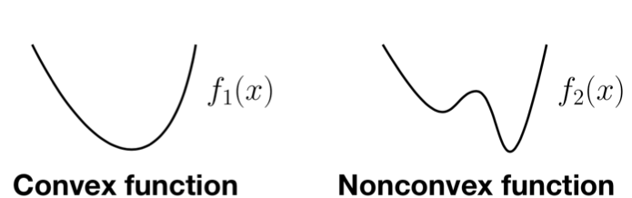
Convexity¶

Originally, researchers distinguished between linear (easy) and nonlinear (hard) problems, but in 80s and 90s it became clear that this wasn’t the right distinction; the key difference is between convex and non-convex problems.

First, we need to know the definition of convex sets and convex functions:

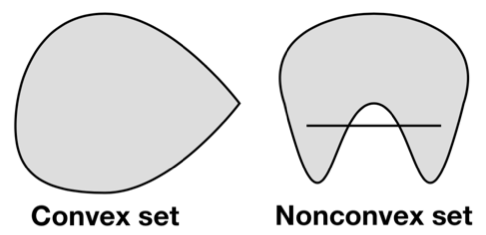
Convex sets¶

A set $\mathcal{C}$ is convex if and only if $$\forall x,y\in\mathcal{C},\theta\in[0,1]\;\;\;\;\;\theta x+(1-\theta)y\in\mathcal{C}.$$

For example, the following sets are convex:

• $\mathbb{R}^n$ for all non-negative integers $n$
• All intervals $[l,r]$ in $\mathbb{R}$
• Linear equalities $\{x|x\in\mathbb{R}^n,Ax=b\}$ for all $m\times n$ matrices $A$ and all m-dimensional vectors $b$
• Intersection of any number of convex sets
• The set $\{x|x\in\mathbb{R}^2,x_1\ge0,x_2\ge0,x_1\cdot x_2\ge1\}$ (it is the area above the function $f(x)=\frac{1}{x}$)

Note that the union of any number of convex sets need not be convex. (Consider the union of two disjoint circles in $\mathbb{R}^2$.)

Convex functions¶

A function $f:\mathbb{R}^n\rightarrow\mathbb{R}$ is convex if and only if it never curves downward. The formal definition is as follows:

$$\forall x,y\in\mathbb{R}^n,\theta\in[0,1]\;\;\;f(\theta x+(1-\theta)y)\le\theta f(x)+(1-\theta)f(y)$$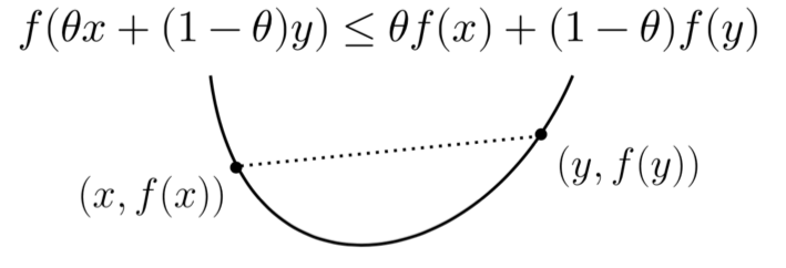

If the function $f$ is convex, we call $-f$ concave, and if $f$ is both convex and concave, then it is an affine function is of the form $$f(x)=\sum^{n}_{i=1}a_ix_i+b.$$

Examples of convex functions are:

• $f(x)=\exp(x)=e^x$
• $f(x)=-\log(x)$ subject to $x>0$
• Euclidean norm and its square: $f(x)=\lVert x\rVert^2_2\equiv x^Tx\equiv\sum^n_{i=1}x^2_i$ and $f(x)=\lVert x\rVert_2\equiv \sqrt{x^Tx}\equiv\sqrt{\sum^n_{i=1}x^2_i}$
• Weighted sum of convex functions with non-negative weights: $$f(x)=\sum^m_{i=1}w_i\cdot f_i(x)$$ where $w_i\ge0$ and $f_i$ are convex.

A simple test for determining the convexity of a function is known as the second-order convexity condition and is as follows:

• $f:\mathbb{R}\rightarrow\mathbb{R}$, is convex if and only if its second derivative is non-negative. #### Proof: Assume $f(ta+(1-t)b)\le tf(a)+(1-t)f(b)$ for all $a,b\in\mathbb{R},t\in[0,1]$. Let $t=\frac{1}{2},a=x-h,b=x+h$. We have: $$f(x)\le\frac{1}{2}f(x-h)+\frac{1}{2}f(x+h)\\\Rightarrow f(x+h)-2f(x)+f(x-h)\ge0$$ (Note that $f''(x)=\lim_{h\to0}\frac{f(x+h)-2f(x)+f(x-h)}{h^2}.$)

Now assume $f''(x)\ge0$ for all $x\in(-\infty,\infty)$. Using the first-order Taylor series expansion of $f$ around $x_0$ we have: $$f(x)=f(x_0)+f'(x_0)(x-x_0)+\frac{f''(x^*)}{2}(x-x_0)^2$$ for some $x^*$ between $x$ and $x_0$. The last term is always positive because of the hypothesis. Setting $x_0=\lambda x_1+(1-\lambda)x_2$, for $x=x_1$ we get: $$f(x_1)\ge f(x_0)+f'(x_0)((1-\lambda)(x_1-x_2)).$$ For $x=x_2$ we get: $$f(x_2)\ge f(x_0)+f'(x_0)(\lambda(x_2-x_1)).$$ Now we can conclude that $$f(x_0)\le\lambda f(x_1)+(1-\lambda)f(x_2)$$ and the proposition is proven.

• $f:\mathbb{R}^n\rightarrow\mathbb{R}$, is convex if and only $\mathbf{H}_f(x)$ (its Hessian matrix) is positive semi-definite at all $x\in\mathbb{R}^n$

Proof¶

Lemma: $f:\mathbb{R}^n\rightarrow\mathbb{R}$ is convex if and only if $g(t)=f(x_0+tu)$ is convex for every $x_0,u\in\mathbb{R}^n$ (the function is convex in every direction). We have $g''(t)=u^T(\mathbf{H}_f(x_0+tu))u\ge0$ for all $x_0$ and $u$, so $\mathbf{H}_f(x)$ must be positive semi-definite for all $x$.

Using the second-order convexity test, we can easily show that:

• $f(x_1,x_2)=x_1\cdot x_2$ is not convex.
• $f(x_1,x_2)=x^2_1+x^2_2+x_1x_2$ is convex.

Convex Optimization¶

As you may know, convex optimization problem is an optimization problem in which the objective function is a convex function and the feasible set is a convex set. Now let's examine some useful properties:

• every local minimum is a global minimum
• the optimal set is convex
• if the objective function is strictly convex, then the problem has at most one optimal point

In fact, many of search algorithms find the local optima, and that's why the first property is the key point that enable us to tackle these types of problems to find the global optima solutions. Now let's go through its proof:

Assume there exists $x_0$ such that $f(x_0)<f(x_∗)$ where $x_*$ is the local optima of the function. Then for any $t∈(0,1]t∈(0,1]$ we have: $$f(Z) = f((1−t)x_∗+tx_0)≤(1−t)f(x_∗)+tf(x_0)$$$$<(1−t)f(x_∗)+tf(x_∗)$$$$=f(x_∗)$$ $$\Longrightarrow $$$$f(Z) < f(x_*) $$ Now note that $Z$ is lying on the line which connects $x_0$ and $x_*$. Therefore, if $Z$ is chosen very close to $x_*$, the $f(Z)it $ must be greater than $f(x_*)$ due to local optimality of $x_*$ which means: $$f(Z) \ge f(x_*)$$ which contradicts to the previous relation. Hence the hypothesis was wrong and the property is proved.

---

Now once we found out this useful property, a good idea can be model our problems to a convex optimization problem through which we can apply various iterative methods like gradient descent to solve the problems.

gradient descent¶

The idea is to take repeated steps in the opposite direction of the gradient (or approximate gradient) of the function at the current point, because this is the direction of steepest descent. Conversely, stepping in the direction of the gradient will lead to a local maximum of that function; the procedure is then known as gradient ascent.

The algorithm is really simple (and effective!!!). Isimple which its pseudocode can be in below:

x  = initilize_point()
for EPOCHS tims repeat:
    x -=  learning_rate * gradient(f(x))

n fact, the value of $f$ is decreasing in each iteration. The proof is straight forward as it is illustrated in below: By taylor exapansion of a function $f$ we have: $$f(x+v) = f(x) + \nabla_x f(x)^Tv + O(||v||_2^2)$$ Now choose $v$ to be multiplication of gradient i.e. $-\alpha\nabla_x f(x)$. By substituting in the above equation we have: $$= f(x) -\alpha||\nabla_x f(x)||_2^2 + C||\alpha\nabla_x f(x)||_2^2$$$$\le f(x) - (\alpha-\alpha^2C)||\nabla_x f(x)||_2^2 $$ $$< f(x)\blacksquare$$

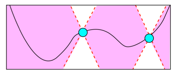
Note that the second relation will only hold for small size of $||\alpha\nabla_x f(x)||_2^2$. Also every $v$ which its inner product with the gradient is less than zero cannot be a good choice because ,as we have seen above, the value of $v$ itself can be effective too. For example see the picture below: If the learning rate (the constant which multiplies to the gradient) is too large convergence might be failed. On the other hand choosing a very small learning rate can slow down the convergence significantly. Therefore, choosing the learning rate can be really critical.

---

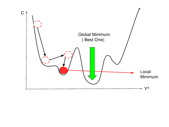So by far we have seen that the gradient descent will converge toward the local minimum (see the figure above to see the importance of starting point in non-convex functions). Now let's go through some examples: consider the function $f = x_1^2+x_2^2 + 2x_1 + x_1x_2$. we have: $$\nabla_{x_1}f = 2x_1 +2 + x_2 = A(x)$$$$\nabla_{x_2}f = 2x_2 + x_1 = B(x)$$$$x_{new_1} = x_1 -\alpha A(x) $$$$x_{new_2} = x_2 -\alpha B(x)$$ and obviously $x_{new} = (x_{new_1}, x_{new_2})$.